>	with(plots):

 

We'll look at this cone; the factor of 5/3 is just to make the aspect ratio look nice as we graph it. 

>	f:=(x,y)->5-5*sqrt(x^2+y^2)/3;

 

(1)

 

So the graph of the cone is (ooo, aaaah): 

>	fig[1]:=plot3d(f(x,y),x=-3..3,y=-3..3,axes=normal,view=[-4..4,-4..4,0..6],numpoints=1000): fig[1];

 

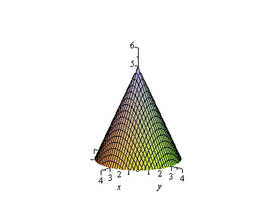z=f(x,y) 

Note that while we've thought of this as a surface here, we can equally think about it as a parametrically defined surface, e.g. with 

   , 

with , , and or we could instead take 

with and .  As an example, let's graph the latter before going on: 

>	plot3d([u*cos(v),u*sin(v),5-5*u/3],u=0..3,v=0..2*Pi,axes=normal,view=[-4..4,-4..4,0..6],numpoints=1000,labels=[x,y,z]);

 

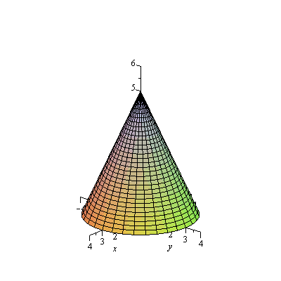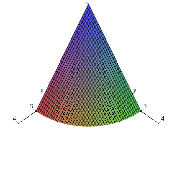
Note how the grid curves change in this case: they have constant or theta constant, instead of and constant.  Next let's just regraph the part of the cone in the first octant. 

>	fig[2]:=plot3d(f(x,y),x=0..3,y=0..3,axes=normal,view=[0..4,0..4,0..5],numpoints=1000,labels=[x,y,z]): fig[2];

 

And then take off the grid lines for a moment, so that we have a cleaner view of the surface. 

>	pl:=plot3d(f(x,y),x=0..3,y=0..3,axes=normal,view=[0..4,0..4,0..5],style=patchnogrid,numpoints=1000): fig[3]:=pl:

 

>	display(pl);

 

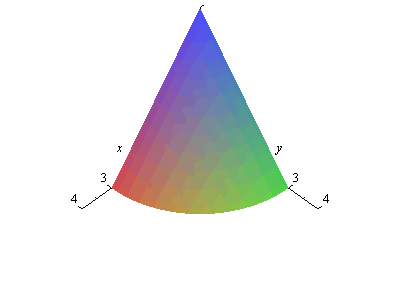z=f(x,y), in the first octant 

Next, we look at a small area element in the -plane (that is, thinking parametrically, a small element in the parameter domain): 

>	h:=0.3: x0:=1: y0:=1: da:=spacecurve({[x0+h,y0+t,0],[x0+t,y0+h,0]},t=0..h,thickness=3,color=red): dx:=spacecurve({[x0+t,y0,0]},t=0..h,thickness=3,color=blue): dy:=spacecurve({[x0,y0+t,0]},t=0..h,thickness=3,color=green):

 

>	fig[5]:=display(pl,da,dx,dy,numpoints=1000): fig[5];

 

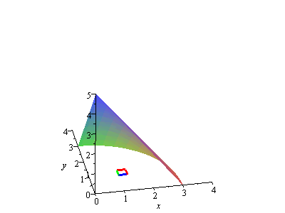z=f(x,y), with dA on the xy-plane (dx=blue, dy=green) 

(To see the area element under the surface, we have to rotate it around so that we're looking from behind.)  Then, the corresponding area element on the surface is 

>

ds:=spacecurve({[x0+h,y0+t,f(x0+h,y0+t)],[x0+t,y0+h,f(x0+t,y0+h)]},t=0..h,thickness=3,color=red): dsx:=spacecurve({[x0+t,y0,f(x0+t,y0)]},t=0..h,thickness=3,color=blue): dsy:=spacecurve({[x0,y0+t,f(x0,y0+t)]},t=0..h,thickness=3,color=green): vert:=spacecurve({[x0,y0,f(x0,y0)*t],[x0+h,y0,f(x0+h,y0)*t],[x0,y0+h,f(x0,y0+h)*t],[x0+h,y0+h,f(x0+h,y0+h)*t]},t=0..1,thickness=2,color=red):

 

>	proj:=display(pl,da,dx,dy,ds,dsx,dsy,vert,numpoints=1000): fig[4]:=display(pl,ds,dsx,dsy,numpoints=1000): fig[6]:=proj: display(proj);

 

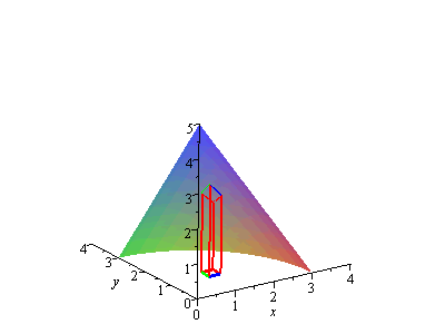z=f(x,y), with dA on the xy-plane and projection to the surface 

Now, at this point we know that , the little area element on the surface, is the projection of the area element in the -plane (or, domain) onto the surface.  It's also a small paralellogram, so we can find its area by looking at the magnitude of the cross product of two vectors that extend along two of the sides of the paralellogram: that is, we know 

But why are the vectors along the two sides of the parallelogram  and ?  The following looks at why that is.  If we zoom in on the surface area element and put the vectors on the two sides, we have 

>	vecx:=arrow([x0,y0,f(x0,y0)],[h,0,h*subs(x=x0,y=y0,diff(f(x,y),x))],color=blue): vecy:=arrow([x0,y0,f(x0,y0)],[0,h,h*subs(x=x0,y=y0,diff(f(x,y),y))],color=green):

 

>	fig[7]:=display3d(proj,vecx,vecy,view=[(x0-.5)..(x0+.5),(y0-.5)..(y0+.5),1.5..3]): fig[7];

 

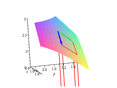the same, showing the vectors along two sides of dS 

What are these vectors?  The blue vector points along the side of the parallelogram that is projected up from the side of the area element in the -plane, so, if is the parameterization of the surface, it points from to .  That is, the blue vector is the vector 

Similarly the green vector is just , and we get the desired result for .