Gavin's DiffEq Class Clarification: Feb 23

Ok, let's look at an example. We'll consider the differential equation
y' = c + y².
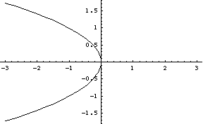
Equilibrium solutions are when y' = 0, or c + y² = 0. This says that y = +/-sqrt(-c). What does this look like? If we just plot it in Mathematica, we see

Plot[{Sqrt[-c], -Sqrt[-c]}, {c,-3,3}];

So it looks like if we look at a value of c <0 we have two equilibrium solutions, while for values larger than 0 there aren't any. This means that we have to worry about two general regions: when c<0, and when c>0. These are the different values of c that we want to consider in our analysis, because they are the regions in which things are different.

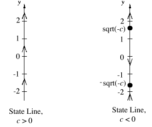
Before actually trying to do a bifurcation diagram, let's think about what our state lines tell us. If c>0, we can see that y' = c + y² > 0, because the right-hand side is the sum of two positive numbers. Thus in this case the state line (with no equilibria) is pretty easy to draw:

If c < 0, then y' = -|c| + y², so if y² >|c| we have y' > 0, and the solution has positive slope (is moving upwards). Similarly, if y² <|c| the solution has negative slope and is moving down, as shown in the second state line above.

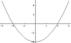
Note that we could draw the second state line by choosing a value for c and then seeing what happens -- for example, if c = -4, then we have y' = -4 + y². The right-hand side of this is

Plot[-4+y^2, {y,-3,3}];

so for y < -2 the derivative is positive, for -2 < y < 2 it is negative and for y > 2 it's positive again -- as shown in the state line above.

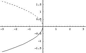
Finally, the bifurcation diagram is the plot of the equilibrium solutions that we have at the top of the page, with solid and dashed lines indicating attracting and repelling equilibrium solutions. As shown in the state lines, the bottom one is an attractor and the top a repeller:

Plot[{Sqrt[-c], -Sqrt[-c]}, {y,-3,3}, PlotStyle->{Dashing[{0.01,0.02}], GrayLevel[0]}];