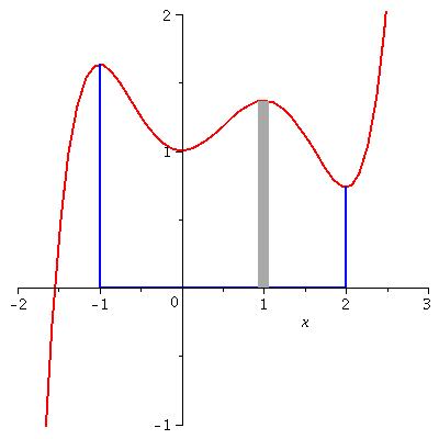
>	with(plots):

 

>	p1:=plot( x^5/5 - x^4/2 - x^3/3 + x^2 + 1, x=-2..3, view=-1..2, thickness=2 ):

 

>	p2:=plot( 0, x=-1..2, thickness=2, color=blue ):

 

>	p3:=plot([-1,t,t=0..49/30], thickness=2, color=blue ):

 

>	p4:=plot([2,t,t=0..11/15], thickness=2, color=blue ):

 

>	p5:=plot([1,t,t=0..41/30], thickness=10, color="DarkGrey"):

 

>	display(p1,p2,p3,p4,p5);

 

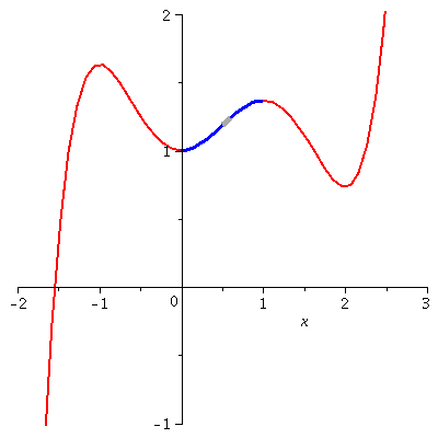
>	p6:=plot( x^5/5 - x^4/2 - x^3/3 + x^2 + 1, x=0..1, view=-1..2, thickness=3, color=blue ):

 

>	p7:=plot( x^5/5 - x^4/2 - x^3/3 + x^2 + 1, x=0.5..0.6, view=-1..2, thickness=5, color="DarkGrey" ):

 

>	display( p1, p6, p7 );

 

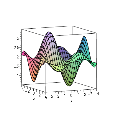
>	q1:=plot3d( sin(x)*(cos(y)+0.5)+2, x=-4..4, y=-4..4, axes=boxed ):

 

>	display3d(q1);

 

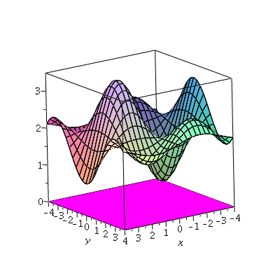
>	q2:=plot3d( 0, x=-4..4, y=-4..4, axes=boxed, style=surface, color="Magenta" ):

 

>	display3d( q1, q2 );

 

>

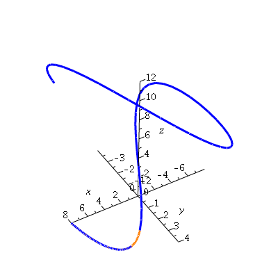
f1:=t->[8*cos(t),4*sin(2*t),2*t]: sc1:=spacecurve(f1(t),t=0..0.25*Pi,color=blue,thickness=3,axes=normal,view=0..12): sc2:=spacecurve(f1(t),t=(0.25*Pi+0.25)..2*Pi,color=blue,thickness=3,axes=normal,view=0..12): sc3:=spacecurve(f1(t),t=0..0.25*Pi+0.25,color=coral,thickness=3,axes=normal,view=0..12): display3d(sc1,sc2,sc3, labels=[x,y,z]);

 

>