>	with(plots):

 

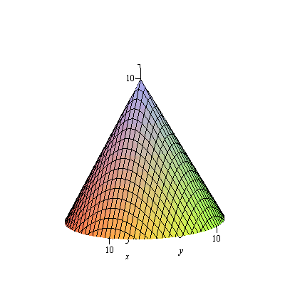
A look (ahead) at projections and the use of cross-products.  First, a nice surface: 

>	f:=(x,y)->10-sqrt(x^2+y^2);

 

(1)

 

>	fig[1]:=plot3d(f(x,y),x=-10..10,y=-10..10,axes=normal,view=[-10..10,-10..10,0..11],numpoints=1000): fig[1];

 

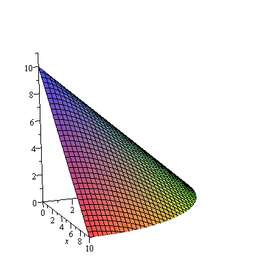
It's convenient to look at only the portion of this in the first octant. 

>	fig[2]:=plot3d(f(x,y),x=0..10,y=0..10,axes=normal,view=[0..10,0..10,0..11],numpoints=1000): fig[2];

 

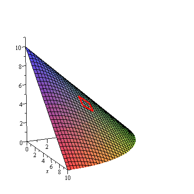
Now suppose that we wanted to find the area of this surface; we might break it into smaller area elements that look like parallelograms, and the area of which are given by a cross-product! 

>

fig[3]:=spacecurve([3+t,4,f(3+t,4)+.1],t=0..1,color=red,thickness=3): fig[4]:=spacecurve([3+t,5,f(3+t,5)+.1],t=0..1,color=red,thickness=3): fig[5]:=spacecurve([3,4+t,f(3,4+t)+.1],t=0..1,color=red,thickness=3): fig[6]:=spacecurve([4,4+t,f(4,4+t)+.1],t=0..1,color=red,thickness=3): display(fig[2],fig[3],fig[4],fig[5],fig[6]);

 

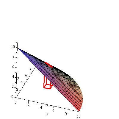
Of course, we would probably prefer to work with a parallelogram in the plane... which requires projecting the parallelogram down to the x-y plane.  And projections are the desmene of the dot product. 

>

fig[7]:=spacecurve([3+t,4,0],t=0..1,color=red,thickness=3): fig[8]:=spacecurve([3+t,5,0],t=0..1,color=red,thickness=3): fig[9]:=spacecurve([3,4+t,0],t=0..1,color=red,thickness=3): fig[10]:=spacecurve([4,4+t,0],t=0..1,color=red,thickness=3): fig[11]:=spacecurve([3,4,t],t=0..f(3,4),color=red,thickness=3): fig[12]:=spacecurve([4,4,t],t=0..f(4,4),color=red,thickness=3): fig[13]:=spacecurve([3,5,t],t=0..f(3,5),color=red,thickness=3): fig[14]:=spacecurve([4,5,t],t=0..f(4,5),color=red,thickness=3): display(fig[2],fig[3],fig[4],fig[5],fig[6],fig[7],fig[8],fig[9],fig[10],fig[11],fig[12],fig[13],fig[14]);

 

>