>	with(plottools): with(plots):

 

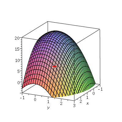
A function giving a hill on which we might walk 

>	f := (x,y) -> 18 - 2*x^2 - 3*y^2;

 

(1)

 

>	p1 := plot3d( f(x,y), x=-1..3, y=-1..3, axes=boxed, view=[-1..3,-1..3,-5..20] ): p2 := sphere( [2,1,f(2,1)], 0.15, color=red, style=patchnogrid): display3d( p1, p2 );

 

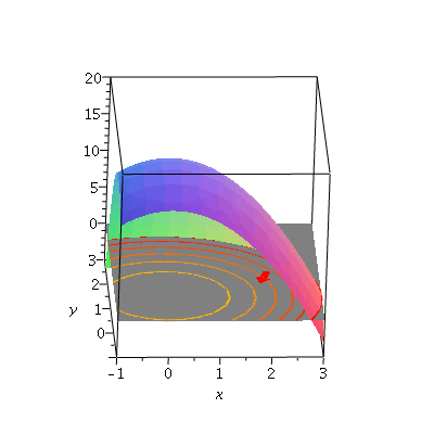
If we look under the hill, we can see the plane, on which we can draw level curves, and can think about a direction v we might move 

>

f1p1:=plot3d( f(x,y), x=-1..3, y=-1..3, axes=boxed, view=[-1..3,-1..3,-5..20], style=patchnogrid ): f1p2a:=plot3d( 0, x=-2..3, y=-2..3, style=patchnogrid, color="Gray" ): f1p2:=contourplot( f(x,y), x=-2..6, y=-2..6, thickness=2, contours=[0,3,6,9,12,15,18] ): q := transform( (x,y)->[x,y,0] ): f1p3:=arrow([2,1,0],[-1,-3,0],color=red,width=[0.15,relative=false],length=[.5,relative=false],head_length=[.2,relative=false]): fr[1]:=display3d( { f1p1, f1p2a, q(f1p2), f1p3 } ): fr[1];

 

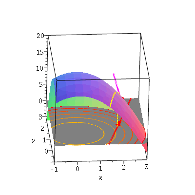
Along the surface, this is the curve shown in yellow; the tangent with the slope of  in the direction of the vector v is shown in magenta. 

>

f2p1:=spacecurve([2-t,1-3*t,0],t=-0.7..0.7,color=red,thickness=3): f2p2:=spacecurve([2-t,1-3*t,f(2-t,1-3*t)],t=-0.5..0.7,color=yellow,thickness=3): f2p3:=spacecurve([2,1,t], t=0..f(2,1), color=yellow, thickness=3): f2p4:=spacecurve([1.84,0.53,t], t=0..f(1.84,0.53), color=yellow, thickness=2): f2p5:=sphere( [2,1,f(2,1)], 0.15, color=red, style=patchnogrid): du := 26/sqrt(10): f2p6:=spacecurve( [2-t,1-3*t,f(2,1)+26*t], t=-0.5..0.5, color=magenta,thickness=3,view=[-1..3,-1..3,-5..20] ): fr[2]:=display3d({ f1p1, f1p2a, q(f1p2), f1p3,f2p1,f2p2,f2p3,f2p4,f2p5,f2p6} ): fr[2];

 

>

 

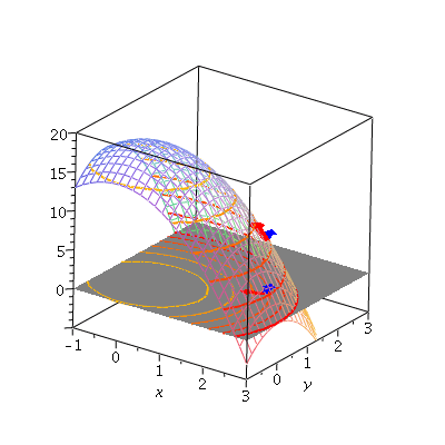
Note that if we point the vector u along the level curve, the derivative is zero, and if we point it perpendicular to the level curve, the derivative is the largest possible value. 

>

f3p0:=plot3d(f(x,y), x=-1..3, y=-1..3, style=wireframe, axes=boxed, view=[-1..3,-1..3,-5..20]): f3p1:=arrow([2,1,0],[-8,-3,0],color=red,width=[0.15,relative=false],length=[.5,relative=false],head_length=[.2,relative=false]): f3p2:=arrow([2,1,0],[-3,8,0],color=blue,width=[0.15,relative=false],length=[.5,relative=false],head_length=[.2,relative=false]): f3p3:=arrow([2,1,f(2,1)],[-4,-3,50],color=red,width=[0.15,relative=false],length=[2,relative=false],head_length=[.2,relative=false]): f3p4:=arrow([2,1,f(2,1)],[-3,8,0],color=blue,width=[0.15,relative=false],length=[.5,relative=false],head_length=[.2,relative=false]): r := transform( (x,y)->[x,y,f(x,y)] ): fr[3]:=display3d({ f3p0, f1p2a, q(f1p2), r(f1p2), f3p1, f3p2, f3p3, f3p4 } ): fr[3];

 

>