>	with(plottools): with(plots):

 

A nice function with which to work 

>	f:=(x,y)->2*x^2+3*y-x*y^2;

 

(1)

 

Note that critical points are where 

>	solve( { diff(f(x,y),x)=0, diff(f(x,y),y)=0 }, {x,y} );

 

(2)

 

That isn't very enlightening; let's get a numerical value: 

>

evalf(%);

 

(3)

 

>

 

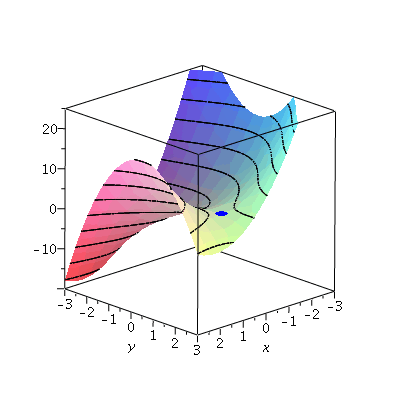
Now let's plot this point and the curve together to see that the critical point is, in fact, a saddle point: 

>	a:=plot3d(f(x,y),x=-3..3,y=-3..3,axes=boxed,style=patchcontour):

 

>	cp:=display(sphere([6^(2/3)/4,6^(1/3),f(6^(2/3)/4,6^(1/3))],0.2,color=blue),style=patchnogrid): ca:=display(sphere([0,0,f(0,0)],0.2,color=black),style=wireframe):

 

>	display(a,cp,ca,view=[-3..3,-3..3,-20..25]);

 

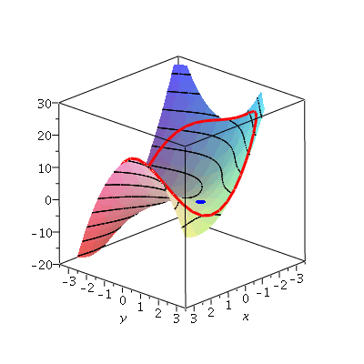
Next, suppose that we are constrained to consider only function values on (or within) the curve 

>	b:=spacecurve([3*cos(t),3*sin(t),f(3*cos(t),3*sin(t))+.5],t=0..2*Pi,color=red,thickness=3): display(a,b,cp,view=[-3.5..3.5,-3.5..3.5,-20..30]);

 

The critical points on the border are where  is: 

>	cpsol := solve( -36*cos(t)*sin(t) + 9*cos(t) + 27*(sin(t))^3 - 54*(cos(t))^2*sin(t) = 0, t ): evalf( cpsol );

 

(4)

 

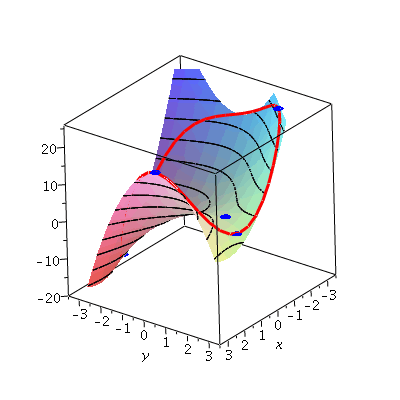
(note that only the first four of these are real-valued).  Plugging these into the expressions for , , and then , we get the points: 

>	bp1:=display(sphere([1.08,-2.80,-14.52+.5],0.2,color=blue),style=patchnogrid):

 

>	bp2:=display(sphere([2.98,0.30,18.45+.5],0.2,color=blue),style=patchnogrid):

 

>	bp3:=display(sphere([1.32,2.70,1.99+.5],0.2,color=blue),style=patchnogrid):

 

>	bp4:=display(sphere([-2.20,2.03,24.95+.5],0.2,color=blue),style=patchnogrid):

 

>	display(a,b,cp,bp1,bp2,bp3,bp4,view=[-3.5..3.5,-3.5..3.5,-20..26]);

 

From this, we can see the absolute maximum and minimum! 

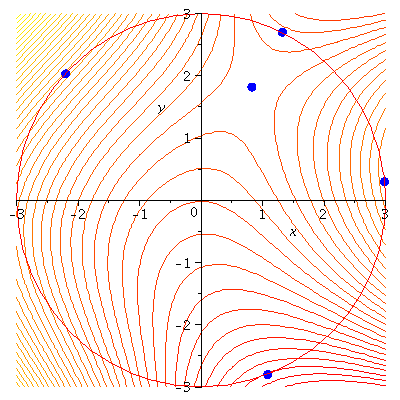
By plotting the contour plot for  and the constraint  together, we can see that the critical points on the boundary occur where we expect them to from the Method of Lagrange Multipliers: where  is parallel to , that is, when : 

>	fcp:=contourplot(f(x,y),x=-3..3,y=-3..3,axes=normal,contours=45,grid=[40,40]):

 

>	cpp1:=display(point([1.08,-2.80]),color=blue,symbol=solidcircle,symbolsize=20):

 

>	cpp2:=display(point([2.98,0.30]),color=blue,symbol=solidcircle,symbolsize=20):

 

>	cpp3:=display(point([1.32,2.70]),color=blue,symbol=solidcircle,symbolsize=20):

 

>	cpp4:=display(point([-2.20,2.03]),color=blue,symbol=solidcircle,symbolsize=20):

 

>	cpp5:=display(point([6^(2/3)/4,6^(1/3)]),color=blue,symbol=solidcircle,symbolsize=20):

 

>	fbp:=plot([3*cos(t),3*sin(t),t=0..2*Pi],axes=normal):

 

>	display(fcp,cpp1,cpp2,cpp3,cpp4,cpp5,fbp);

 

In this,  will be everywhere perpendicular to the circle (given by ), and  will be everywhere perpendicular to the level curves. 

>