>	with(plottools): with(plots):

 

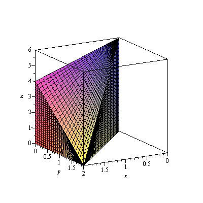
Let's consider a 3D region 

>	p1:=plot3d([x,y,6-x-2*y],x=0..2,y=0..x,axes=boxed,labels=[x,y,z]): p2:=plot3d([2,y,z],y=0..2,z=0..4-2*y): p3:=plot3d([x,x,z],x=0..2,z=0..6-3*x): fr[1]:=display3d(p1,p2,p3,orientation=[60,75]): fr[1];

 

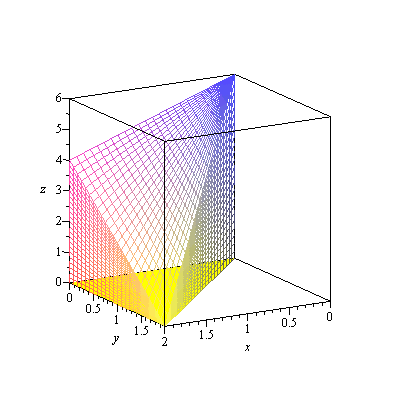
Some more detail: we'll first make the figure a wireframe, so that we can see through it.  We then put in the region that we'd integrate over for the double integral in 

   , 

as a yellow region in the -plane, and then put in possible vertical and horizontal slices before finally adding the "slice" in . 

>

fr[2]:=display3d(p1,p2,p3,style=wireframe,orientation=[60,75]): p4:=plot3d([x,y,0],x=0..2,y=0..x,style=surface,color=yellow): fr[3]:=display3d(fr[2],p4,orientation=[60,75]): fr[4]:=display3d(fr[3],orientation=[-90,0]): toxy:=transform( (x,y) -> [x,y,0.025] ): p5:=plot(x,x=1.5..1.6,filled=true,color=blue): fr[5]:=display3d(fr[4],toxy(p5)): p6:=plot([x,1.25,x=1.25..2],thickness=10,color=blue): fr[6]:=display3d(fr[4],toxy(p6)): p7:=spacecurve([1.55,1.25,t],t=0..6-1.55-2*1.25,color=blue,thickness=10): fr[7]:=display3d(fr[3],toxy(p6),p7): p8:=spacecurve([1.55,1.25,t],t=0..1,color=blue,thickness=10): p9:=spacecurve([1.55,1.25,t],t=1.2..6-1.55-2*1.25,color=blue,thickness=10): p10:=spacecurve([1.55,1.25,t],t=1..1.2,color=green,thickness=10): fr[8]:=display3d(fr[3],toxy(p6),p8,p9,p10): display3d(seq(fr[i],i=1..8),insequence=true);

 

More slowly:  the region is 

>	display3d(fr[3]);

 

or 

>	display3d(fr[4],orientation=[-90,0]);

 

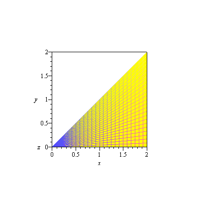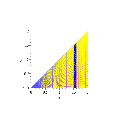
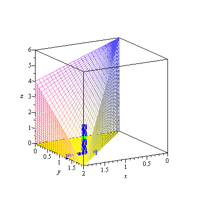
so that vertical slices are 

>	display3d(fr[5],orientation=[-90,0]);

 

and, rotating back and showing the vertical slice and volume element , we have 

>	display3d(fr[8]);

 

>