>	with(plottools): with(plots):

 

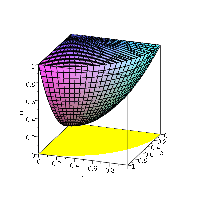
A corner planter, with the projection into the -plane shown in yellow. 

>

p1 := plot3d( [r*cos(t),r*sin(t),1], r=0..1, t=0..Pi/2, axes=boxed, labels=[x,y,z] ): p2 := plot3d( [r*cos(t), r*sin(t), r^2], r=0..1, t=0..Pi/2, axes=boxed, labels=[x,y,z] ): p3 := plot3d( [r*cos(t),r*sin(t),0], r=0..1, t=0..Pi/2, axes=boxed, labels=[x,y,z], style=patchnogrid, color=yellow ): display3d( p1, p2, p3, orientation=[20,70] );

 

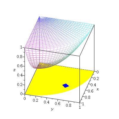
Then, if we use polar coordinates, we have the small area element shown in blue: 

>

p1a := plot3d( [r*cos(t),r*sin(t),1], r=0..1, t=0..Pi/2, axes=boxed, labels=[x,y,z], style=wireframe ): p2a := plot3d( [r*cos(t), r*sin(t), r^2], r=0..1, t=0..Pi/2, axes=boxed, labels=[x,y,z], style=wireframe ): p4 := plot3d( [r*cos(t),r*sin(t),0.01], r=0.8..0.9, t=Pi/4..Pi/4+.1, axes=boxed, labels=[x,y,z], style=patchnogrid, color=blue ): display3d( p1a, p2a, p3, p4, orientation=[15,55] );

 

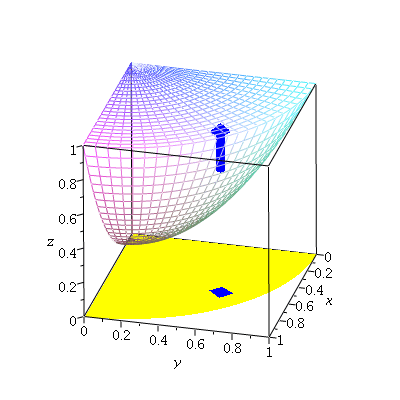
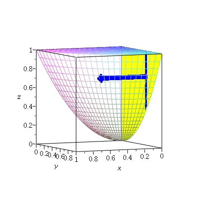
And for each of these regions, the range of values is shown by the arrow: 

>	p5 := arrow([.85*cos(Pi/4+.05),.85*sin(Pi/4+.05),.85^2],[0,0,1],color=blue, width=[0.05,relative=false], length=[1-.85^2,relative=false], head_length=[.05,relative=false]): display3d( p1a, p2a, p3, p4, p5, orientation=[15,55] );

 

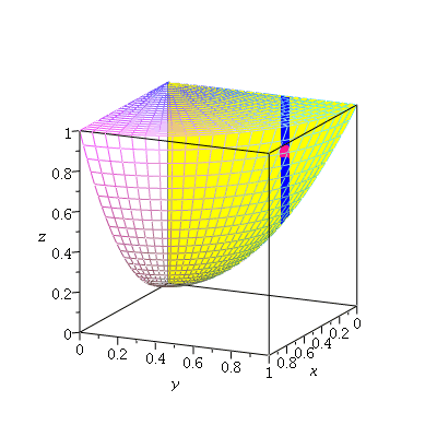
Now, suppose we project the surface into the -plane instead: we have the projection shown in yellow, with a corresponding vertical slice (blue) and small area element (in red). 

>

p6 := plot3d( [0, y, z], z=y^2..1, y=0..1, style=patchnogrid, color=yellow ): p7 := plot3d( [0.01, y, z], z=y^2..1, y=0.6..0.65, style=patchnogrid, color=blue ): p7a := plot3d( [0.015, y, z], z=0.7..0.76, y=0.6..0.65, style=patchnogrid, color="DeepPink" ): display3d( p1a, p2a, p6, p7, p7a, orientation=[25,75] );

 

Then, at each , the corresponding values are  

>	p8 := arrow([0,.625,.73],[1,0,0],color=blue, width=[0.05,relative=false], length=[sqrt(.73-.625^2),relative=false], head_length=[.05,relative=false]): display3d( p1a, p2a, p6, p7, p7a, p8, orientation=[65,85] );

 

>