>	with(plots):

 

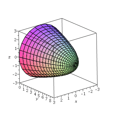
A nice surface: 

>	sp:=plot3d([r*cos(t),9-r^2,r*sin(t)],r=0..3,t=0..2*Pi,axes=boxed,labels=[x,y,z]): sp;

 

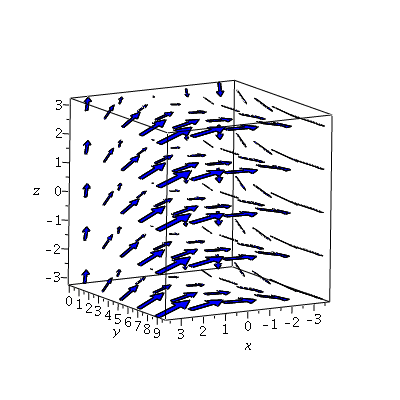
And a nice vector field: 

>	vp:=fieldplot3d([-y,1,x],x=-3..3,y=0..9,z=-3..3,axes=boxed,labels=[x,y,z],arrows=THICK,color=blue,grid=[5,5,5]): vp;

 

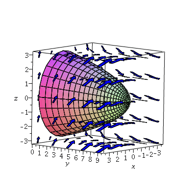
And the two together 

>	display3d(sp,vp);

 

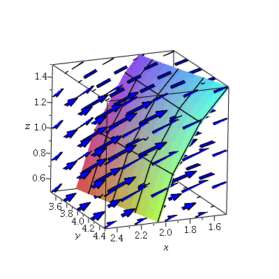
Let's zoom in to see what's going on at a specific point, say (2,4,1) 

>	zs:=plot3d([r*cos(t),9-r^2,r*sin(t)],r=1.75..3.25,t=0...5,axes=boxed,labels=[x,y,z],view=[1.5..2.5,3.5..4.5,0.5..1.5]): zp:=display3d(zs,fieldplot3d([-y,1,x],x=1.5..2.5,y=3.5..4.5,z=0.5..1.5,axes=boxed,labels=[x,y,z],arrows=THICK,color=blue,grid=[5,5,5],view=[1.5..2.5,3.5..4.5,0.5..1.5])): zp;

 

Exactly at the point (2,4,1), the vector field points in the direction 

and a normal to the surface is 

The unit normal is 

That is: 

>

fvec := arrow({[[2,4,1],[-4,1,2]]},length=[.5,relative=false],color=blue): nvec := arrow({[[2,4.098,.95],[-4,-1,-2]]},length=[.5,relative=false],color=red): fvnorm := arrow({[[2,4,1],[-4,-1,-2]]},length=[11/(2*(21)),relative=false],width=[.025,relative=false],color="Purple"): display3d(zs,fvec,nvec,fvnorm);

 

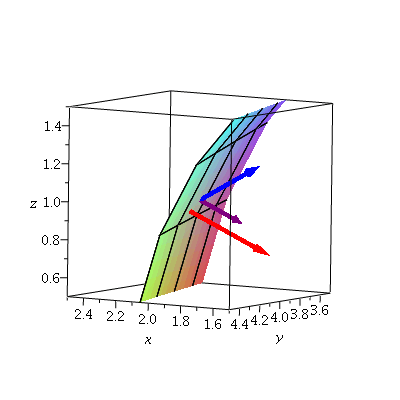The purple vector is the component of F that is pointing through (normal to) the surface.  The red vector is the normal to the surface, moved to the side a little so that it doesn't overwrite the purple vector. 

Then, when we integrate over the surface, we're adding up the length of the component of F in the direction through the surface times the area: thus, if F is a velocity field (measured in m/s), we get a flux of /s: a volume flow-rate through the surface. 

>