>	with(plots):

 

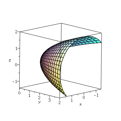
We'll consider a surface that consists of part of a parabaloid: 

>	p1:=plot3d([u*cos(v),u^2,u*sin(v)], u=0..2, v=-Pi/4..3*Pi/4, axes=boxed,labels=[x,y,z]): p1;

 

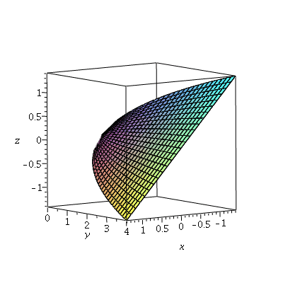
...and part of a plane: 

>	p2:=plot3d([u,v,-u],u=-sqrt(v/2)..sqrt(v/2),v=0..4,axes=boxed,labels=[x,y,z]): p2;

 

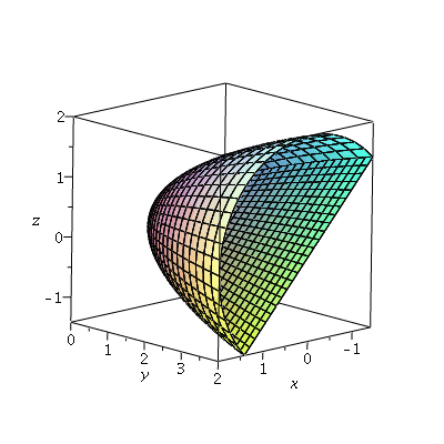
So the full surface is given by the combination of these: 

>	p3:=spacecurve([2*cos(t),4.01,2*sin(t)],t=-Pi/4..3*Pi/4,color=blue,thickness=5): p4:=spacecurve([x,4.01,-x],x=-sqrt(2)..sqrt(2),color=blue,thickness=5):

 

>	display3d(p1,p2);

 

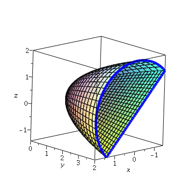
Then the boundary of the surface is the uncovered edge, shown in blue: 

>	display3d(p1,p2,p3,p4);

 

We're looking at Stokes' theorem, so we're interested in finding 

which is equal to the line integral 

We're looking at , for which  The curl is 

>	p5:=fieldplot3d([0,-z,2*x*y],x=-2..2,y=0..4,z=-2..2,axes=boxed,arrows=THICK,grid=[5,5,5]): p5;

 

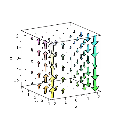and the vector field is 

>	p6:=fieldplot3d([2*x,x^2*y,-x*z],x=-2..2,y=0..4,z=-2..2,axes=boxed,arrows=THICK,grid=[5,5,5]): p6;

 

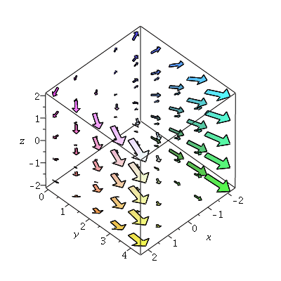This shows the curl of the vector field along with the surface; it isn't really obvious what the surface integral  

is from looking at it. 

>	display3d(p1,p2,p5);

 

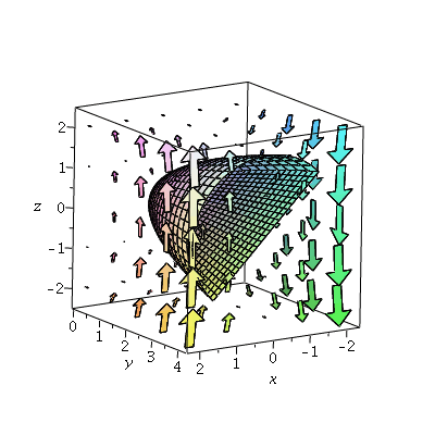Then we can also show the surface with the vector field F.  Here we're interested in the integral 

on the (blue) boundary. 

>	display3d(p1,p2,p3,p4,p6);

 

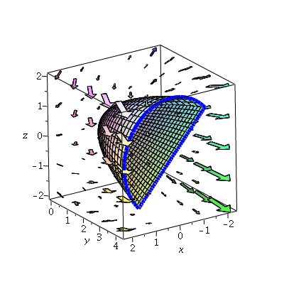It's easier to see what's going on with this by taking advantage of the fact that the boundary is planar (it lives in the plane ).  So we can graph just the boundary and the and components of the vector field to see what the line integral will be like.  Note that we're traversing this counter-clockwise as we see it in the 3D figure above, which in the -plane (below) looks like a clockwise traversal, because we're looking at the curve from behind to make the axis point to the right. 

>	p7:=fieldplot([2*x,-x*y],x=-2..2,y=-2..2): p8:=plot(-x,x=-sqrt(2)..sqrt(2),color=blue,thickness=3): p9:=plot([2*cos(t),2*sin(t),t=-Pi/4..3*Pi/4],color=blue,thickness=3): display(p7,p8,p9);

 

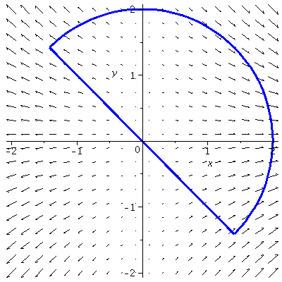(From this, it looks as if the line integral should be positive.) 

>